Comments on the Listing of Compute Derivatives Contracts¹

We appreciate the opportunity to comment on the Commodity Futures Trading Commission's Request for Comment on the Listing of Compute Derivatives Contracts. The Commission cites an earlier version of our paper, (Early) AI Compute Asset Pricing (Bandi and Su, 2026), in its request. We now provide a revised version of that work and additional considerations regarding compute index construction. The updated version of our paper is available here.

For conciseness, we summarize our principal conclusions below.

1. Technological obsolescence. Individual hardware configurations becoming obsolete need not prevent a viable futures market. Contracts can reference specific configurations, with contracts on new configurations introduced as they become available. For each configuration, the term structure can reflect expected obsolescence.

2. Service heterogeneity. Even for a given hardware configuration, the economic value of a GPU-hour can differ across providers because of, e.g., form factor, interconnectivity, and network specifications. A clearly specified reference, or “par”, service may define the underlying, with transparent price adjustments for deviations from the “par” characteristics.

3. OTC transactions and reproducibility. A settlement index should be simple and reproducible from verifiable transactions. A trade-reporting infrastructure that records transactions while protecting privacy can support this objective. Where transaction liquidity is insufficient, firm, binding quotes from a contributor panel could supplement the inputs. Nonbinding indicative quotes should be identified separately and their role in validation and weighting made transparent.

4. Manipulation resistance. In a simple model, below, we suggest that regulators could use unusually large net, settlement-linked futures exposures as a screening signal for closer scrutiny. The model’s exposure threshold should, however, only serve as an illustrative benchmark—not as a validated all-encompassing rule for detecting manipulation. The model also highlights index-design choices that can reduce incentives to distort settlement, including broad and transparent survey coverage, carefully chosen contributor weights, trimming extreme observations, and averaging prices over the settlement period. These safeguards involve trade-offs: weighting affects both manipulation incentives and representativeness, while averaging may reduce manipulation sensitivity but increase basis risk for users exposed near expiry. Because the suggested threshold rests on stylized assumptions about price distortion, economic costs, and exposure, it should inform surveillance and index-design due diligence. It should not be viewed as replacing documented evidence of misconduct or a well-calibrated regulatory standard.

We emphasize that our objective is not advocacy. Our contribution and interests are technical. While we do not believe that compute's distinctive features are an insurmountable obstacle to a viable futures market, compliance with the IOSCO principles requires care and due diligence.

Section 1 develops a simple model of manipulation incentives and its implications for regulation and index construction. Section 2 considers benchmark representativeness, the usefulness of a contract covering a defined market segment, and the risks of over-interpreting its price signals.

1. A simple model of compute index manipulation: implications for regulation and index construction

We study the potential manipulation of the compute rental index for gains in the futures market, as well as its deterrence, by analyzing the incentives and costs of such manipulation using a rational-choice approach to crime and deterrence (Becker, 1968). The model compares the gain on an index-linked financial position with the economic cost of distorting the index and the expected penalty. Under simplifying assumptions, the model provides an exposure threshold above which distortion is economically profitable, informing regulatory guidelines for monitoring position sizes. It also identifies how various index construction considerations can reduce manipulation incentives, informing the design of manipulation-resistant settlement indices.

Suppose provider $i$ distorts its reported rental price by $x_i$ dollars per GPU-hour for one day. Its profit from such distortion is

$$\label{eq:manipulation-profit} \begin{array}{@{}c@{\;}c@{\;}c@{\;}c@{\;}c@{\;}c@{\;}c@{}} \Pi_i(x_i) & = & q_i\Delta_Y(x_i) & - & C_i(x_i) & - & \text{expected penalty}_{i} \\[2pt] \downarrow & & \downarrow & & \downarrow & & \downarrow \\[2pt] \substack{\text{provider }i\text{'s profit}\\\text{from price distortion }x_i} & & \substack{\text{benefit of index distortion}\\=\text{contract exposure}\\\times\text{index distortion}} & & \substack{\text{economic cost}\\\text{of price distortion}} & & \substack{\text{expected penalty}\\\text{for provider }i} \end{array}$$

(1)

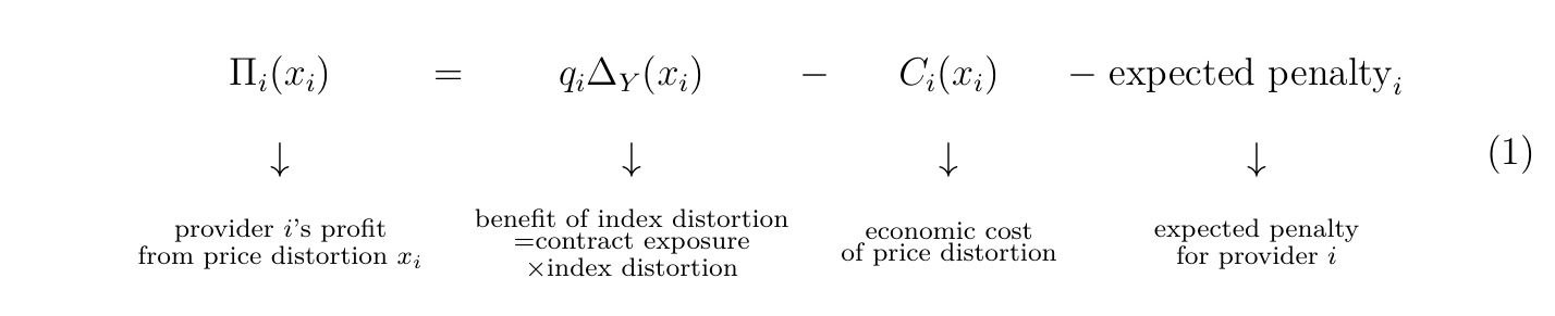
Here, $\Pi_i(x_i)$ is provider $i$'s incremental profit. When $\Pi_i(x_i)>0$, the provider has a net incentive to conduct manipulation. The quantity $q_i$ is provider $i$'s effective settlement-linked financial exposure, positive for a long position and negative for a short; in an application, relevant offsets and related positions should be considered. (Exposure is measured in GPU-hours, thus one unit of $q_i$ represents one GPU-hour of exposure to the index. Under the proposed CME contract specification, one contract represents 730 GPU-hours or, in other words, one GPU-month. The conversion is $Q_i=q_i/730$.) The quantity $\Delta_Y(x_i)$ is the change in the final settlement value induced by provider $i$'s distortion of $x_i$. $C_i(x_i)$ is the economic cost of the one-day reporting distortion, e.g., from charging a suboptimal price in the compute rental market. The final term is the expected penalty due to index manipulation, which is driven by the probability of sanction and punishment conditional on sanction.

Without specifying the details of index construction, Eq. (1) yields the following implications for monitoring financial positions and improving manipulation resistance.

• Financial exposure. Larger exposures $|q_i|$ increase financial benefit and favor distortions. Monitoring unusually large exposures is therefore a relevant consideration. The more detailed quantitative analysis below provides a threshold for the magnitude of $q_i$ above which manipulation is profitable.

• Sensitivity of the settlement index. The financial benefit depends on how strongly an individual reporting distortion changes settlement, as described by $\Delta_Y(x_i)$. A general design objective is to limit the magnitude of $\left|\frac{\partial\Delta_Y(x_i)}{\partial x_i}\right|$ (i.e., the sensitivity of the index to individual price distortions), while preserving the index's ability to represent rental prices. This consideration is relevant to index design choices such as volume weighting, averaging over the settlement month, contributor weight caps, and trimming extreme price inputs (Duffie and Dworczak, 2021).

• Economic cost of distortion. The cost $C_i(x_i)$ depends on the industrial organization of the compute rental spot market and the obligations associated with reported prices. Competition, customer switching, capacity utilization, and execution commitments determine whether manipulation entails forgone revenue, unfavorable transactions, or other economic penalties.

• Legal and institutional environment. The expected monetary punishment depends on the probability of being sanctioned and the sanction, conditional on enforcement. Auditing, surveillance, and legal jurisdiction shape these terms. We take the typical institutional framework for deterring manipulation to be applicable to the compute market. In this sense, the last term in Eq. (1) is not the focus of our simple model, which examines compute-specific issues. Having made this point, legal and institutional deterrents are important.

1.1. Adding details to the model

Next, we introduce simplifying assumptions in order to derive sharper quantitative implications. We follow Duffie and Dworczak (2021), Kumar and Seppi (1992), and Zhang (2022).

1. Assume that settlement is the average of daily observations on the index over month $t$:

   

   $$\label{eq:monthly-settlement} Y_t=\frac{1}{|\mathcal D_t|}\sum_{\tau\in\mathcal D_t}Y_\tau, \qquad Y_\tau=\sum_{i=1}^{N}W_i P_{i\tau}.$$

   (2)

   Here $\mathcal D_t$ is the set of days included in settlement for month $t$ and $|\mathcal D_t|$ denotes the number of days in that set. $Y_t$ is the monthly settlement average, $Y_\tau$ is the daily index, $P_{i\tau}$ is constituent $i$'s reported rental price on day $\tau$, and $W_i>0$ is its weight, with $\sum_{i=1}^{N}W_i=1$. Assume homogeneous GPU services, with $N$ providers contributing to the index. Two examples of how to set the weights are

   

   $$\label{eq:index-weights} W_i=\frac{V_i}{V_{\mathrm{AGG}}} \quad\text{(volume weighting)} \qquad\text{or}\qquad W_i=\frac{1}{N} \quad\text{(equal weighting)},$$

   (3)

   where $V_i$ is the number of continuously rented GPUs supplied by provider $i$ and $V_{\mathrm{AGG}}=\sum_{i=1}^N V_i$ is the total stock of GPUs covered by the index survey sample. Quantities and weights are held fixed. Thus, a price distortion $x_i$ on one specific day changes the settlement value by $\Delta_Y(x_i)=W_i x_i/|\mathcal D_t|$.

2. Assume a linear economic cost, i.e., $C_i(x_i)=24\gamma V_i|x_i|$, where $\gamma>0$ is the economic cost per affected GPU-hour per dollar of price distortion, and assume that the distortion applies throughout the day for 24 hours to all $V_i$ GPUs supplied by provider $i$. The case $\gamma=1$ corresponds to sacrificing one dollar on every affected GPU-hour for a one-dollar price reduction, with rental quantities held fixed. Values $\gamma<1$ describe a cheaper distortion technology. This cost assumption is imposed for the direction of distortion under consideration; upward and downward distortions need not have the same cost in practice.

3. As mentioned, we ignore the expected penalty term to focus on the providers' main trade-off.

Consider a price distortion in the direction favored by the financial position. The marginal profit per additional dollar of distortion in the reported price for one day is

$$\label{eq:marginal-profit} \pi_i\equiv\frac{\partial\Pi_i}{\partial |x_i|} =\frac{|q_i|W_i}{|\mathcal D_t|}-24\gamma V_i.$$

(4)

The pre-penalty threshold for positive marginal gains from the specified manipulation is therefore

$$\label{eq:exposure-cutoff} q_i^{\mathrm M}=\frac{24|\mathcal D_t|\gamma V_i}{W_i}, \qquad \pi_i>0\quad\Longleftrightarrow\quad |q_i|>q_i^{\mathrm M},$$

(5)

where the last condition refers to distortion in the direction favored by the position.

Express exposure in standardized GPU-months as $Q_i=q_i/730$, with one contract-month defined as 730 GPU-hours (a standardized contract unit, not the exact number of hours in every calendar month). This equals the signed number of contracts for a futures contract with a 730 GPU-hour multiplier. The exact threshold in these units is $Q_i^{\mathrm M}=(24|\mathcal D_t|/730)\gamma V_i/W_i$. For the simple benchmark comparisons below, take settlement observations to cover calendar days and use $24|\mathcal D_t|\approx730$. Under this approximation, the threshold simplifies to $Q_i^{\mathrm M}=\gamma V_i/W_i$. Business-day sampling would suggest retaining the factor $24|\mathcal D_t|/730$.²

This is a pre-penalty marginal-incentive threshold for the particular unilateral distortion and cost technology specified above. It is not, by itself, a threshold for the optimal distortion or a general measure of manipulation risk. A provider with net futures exposure $|Q_i|\leq Q_i^{\mathrm M}$ has nonpositive marginal gains from increasing that distortion under the model, before expected penalties. Exposure above the threshold makes the marginal gain positive. This conclusion conditions on an existing financial position and omits the cost of acquiring, financing, or unwinding it.

1.2. Discussion

Total survey size as a monitoring threshold.

Under the volume-weighting scheme, $W_i=V_i/V_{\mathrm{AGG}}$. This scheme would lead to a simple expression:

$$\label{eq:volume-weighted-threshold} Q_i^{\mathrm M}=\gamma V_{\mathrm{AGG}}.$$

(6)

Individual volume $V_i$ cancels out, so the same absolute exposure threshold applies to small and large providers. This cancellation is a consequence of the assumed linear cost, which scales with all $V_i$ GPUs supplied by the provider, and of volume weights proportional to $V_i$. It need not hold if the price distortion affects only a subset of capacity, if reported prices are nonbinding, or if the economic cost does not scale proportionately with supplied volume.

A larger total stock of GPUs covered by the index survey raises the exposure threshold for profitable manipulation. Under this assumption, therefore, broader survey coverage deters manipulation regardless of how the covered stock is distributed across providers.

As a numerical example, suppose the index provider's survey represents a total stock of $V_{\mathrm{AGG}}=10{,}000$ GPUs across all surveyed providers and $\gamma=1$. Under the calendar-day approximation above, any single provider with net futures exposure exceeding 10,000 GPU-months (futures positions of $10{,}000\times730$ GPU-hours) has a positive marginal incentive to manipulate the index unilaterally by changing its reported rental price in the direction favored by its position.

In this example, 10,000 GPU-months is a model-based candidate exposure level for enhanced scrutiny, not a validated regulatory safe harbor or a stand-alone surveillance threshold. The appropriate monitoring level should depend on the index methodology, the quantity actually affected by a provider's price change, the provider's effective settlement-linked exposure (including relevant offsets), and the plausibility of the assumed cost technology.

A lower economic cost of distortion ($\gamma<1$) reduces the model's marginal-incentive threshold.

Distinguishing manipulation-prone positions from ordinary hedging positions.

Next, we compare the manipulation threshold with the position needed to hedge a provider's rental revenue. The goal is to determine the extent to which profitable manipulation requires exposure beyond ordinary hedging needs, and how the distinction between manipulation and legitimate hedging needs depends on the provider's index weight and distortion cost.

For a stylized benchmark, suppose a common price movement changes the provider's rental price and the settlement index equally, and the provider's revenue exposure is $730V_i\Delta p$. A futures position of magnitude $Q_i^{\mathrm H}$ offsets this change when $730Q_i^{\mathrm H}\Delta p=730V_i\Delta p$. Thus, given this benchmark (and the calendar-day approximation), the hedge position and its relation to the manipulation threshold are

$$\label{eq:hedge-comparison} Q_i^{\mathrm H}=V_i, \qquad \frac{Q_i^{\mathrm M}}{Q_i^{\mathrm H}}=\frac{\gamma}{W_i}.$$

(7)

Under this stylized hedge benchmark, when $\gamma=1$ and volume weighting gives a provider a $W_i=V_i/V_{\mathrm{AGG}}=10\%$ index weight, the marginal-manipulation threshold is ten times the benchmark hedge. (This gap may be informative for monitoring, but it is not a universal separation between manipulation-prone positions and legitimate hedges: actual hedge needs depend on revenue sensitivity, contract-index covariance, service mix, and any basis risk.) If the index is highly concentrated ($W_i$ close to one), or if distortion is relatively cheap ($\gamma<W_i$), the model's threshold can approach or fall below the benchmark hedge. Anticipated manipulation profits can themselves encourage over-hedging, as analyzed by Zhang (2022). Suppose we switch to equal weighting. Then $Q_i^{\mathrm M}/Q_i^{\mathrm H}=\gamma N$, so the ratio of the surveillance threshold to the ordinary hedging position is constant across small and large providers, thereby offering an equal proportional buffer for surveillance monitoring. Holding $\gamma$ fixed, surveying more providers (a larger $N$) increases this surveillance buffer ratio.

Index construction method: volume weighting versus equal weighting.

As a general principle within this simple model, volume weighting makes larger providers more susceptible to manipulation, whereas equal weighting makes smaller providers more susceptible. The choice between the two, or a weighting method that lies between these two regimes, depends on the following trade-offs.

If monitoring centers on the absolute size (number of contracts) of the manipulation threshold $Q_i^{\mathrm M}$, volume weighting provides a common surveillance level across providers, as shown in Eq. (6). This result depends on the assumption that the economic cost of distortion ($C_i(x_i)$) also scales with the provider's size ($V_i$). When this assumption does not hold, as may be the case for nonbinding posted prices rather than transaction prices, the benefit of volume weighting is less clear, and a weighting method closer to equal weighting may be considered.

If monitoring instead focuses on distinguishing manipulation-prone positions from ordinary hedging positions, the relevant measure is the ratio $Q_i^{\mathrm M}/Q_i^{\mathrm H}$. Under volume weighting, if one provider accounts for most of the surveyed volume, for example $W_i=V_i/V_{\mathrm{AGG}}=75\%$, its manipulation threshold is only $4/3$ of its ordinary hedge when $\gamma=1$. This leaves little room to distinguish manipulation-prone positions from ordinary hedging positions. Capping very large contributor weights may therefore be useful, moving the weighting toward a more equal allocation.³ Equal weighting sets $W_i=1/N$, so Eq. (7) gives the same ratio $\gamma N$ for every provider. Moving toward equal weighting therefore widens the proportional surveillance buffer for larger providers while narrowing it for smaller providers. This favors more equal weighting when the concern is that a large provider's manipulation threshold lies too close to its ordinary hedge. The trade-off is a lower absolute threshold for smaller providers.

Index construction method: trimming extreme price inputs.

Suppose a trader already has an unusually large exposure that exceeds the threshold for marginally profitable manipulation ($|Q_i|>Q_i^{\mathrm M}$). Under the linear benefit and cost assumptions, its total profit before penalty, $\pi_i|x_i|$, continues to increase with larger distortions $|x_i|$. Within this linear model, the only remaining potential deterrent to ever-larger distortions is the expected penalty: larger distortions may become more conspicuous, increasing the ex-ante probability of sanction and hence the expected penalty.

Trimming extreme price inputs in index construction can provide another channel for deterring ever-increasing manipulation. Trimming would therefore exclude observations in specified lower and upper tails of the price distribution when calculating the index. Once a price change is excluded (and the retained observations and their weights are unchanged), further distortions have no marginal effect on settlement, i.e., $\partial\Delta_Y(x_i)/\partial x_i=0$. Thus, trimming is a reasonable index design choice for limiting manipulation gains from extreme price inputs.

A provider may therefore recognize that trimming can bound its gains, even when $|Q_i|>Q_i^{\mathrm M}$, if the rule bounds the attainable settlement change for that position. This conclusion is conditional: a price input must remain outside the retained set, and the retained observations and weights must not change in response to the distortion. In practice, rank changes, cutoff effects, and changes in the set of retained contributors can make the settlement impact nonzero. If the maximum attainable gain, net of expected penalties, is negative, the manipulation incentive would dissipate.

Index construction method: averaging over the settlement month.

Averaging over the settlement month dilutes the effect of a one-day distortion. Under the model's assumptions, replacing the monthly average with a single-day fixing lowers the threshold by a factor of $| \mathcal D_t|\approx 30$. The dilution is weaker if a distortion can be sustained over multiple settlement days. The trade-off is that an average responds less to prices near expiry and may increase basis risk for users whose exposure is concentrated at that date rather than spread over the settlement month.

2. Considerations regarding representativeness and transparency

Much of compute pricing is currently OTC. If the objective were to obtain a truly representative index which is easily replicable by market participants and auditors, the relevant transactions would have to be readily available. A trade-reporting infrastructure that records transactions while protecting privacy can support this objective. Where transaction liquidity is insufficient, firm, binding quotes from a contributor panel could supplement the inputs; nonbinding indicative quotes should be distinguished and their use in validation and weighting made transparent.

We argue, however, that the first batch of compute futures contracts need not represent the entire compute economy. Given the size of the compute market and the substantial uncertainty surrounding it, financializing a clearly-defined small segment of the compute universe can have substantial economic value by serving the risk-management needs of users and providers in that segment and beyond (through cross-hedging). In other words, contracts need clearly-defined economic exposures and credible settlement benchmarks. Their scope may, however, be more limited than representing the entire compute ecosystem, at least initially.

We further argue that interpreting the first compute futures contracts as representative of a broader market than they actually cover could have unintended consequences. The following channels are conditional risks: they require market participants to treat a narrow futures benchmark as a broad signal and lenders/investors to respond to it. If futures prices are mistakenly treated as a general guide to AI infrastructure investment and financing, they could distort credit decisions and amplify the credit cycle. Two channels from the existing literature help explain this concern. First, a coordination channel can arise when participants care about others' responses as well as fundamentals (Morris and Shin, 2002). Because AI infrastructure financing relies heavily on syndicated loans, private credit, and large debt packages, lenders may look for any forward-looking price anchor. If market participants treat compute futures as a general “health index” for the entire AI sector, compute futures may lead to a coordination trap. Lenders might keep funding marginal projects simply because they think other lenders are looking at the same futures signal and doing the same—until sentiment shifts, leading to a sudden, coordinated freeze. Second, a distinct collateral channel could lead to disruptions (Kiyotaki and Moore, 1997). AI infrastructure is exceptionally capital-intensive, and much of it is debt-financed using the underlying physical assets (hardware, facilities, future cash-flow contracts) as collateral. If a drop in compute futures prices signals falling future utilization or margins, lenders may immediately mark down the value of existing infrastructure collateral. This may trigger margin calls, tighter borrowing limits, forced liquidations, and/or distressed asset sales. Those fire sales then would depress actual asset values further, creating a vicious feedback loop between the financial market and physical capital expenditure. We note, once more, that these channels represent theoretical (tail) risk mechanisms, rather than the likely effect of a well-functioning compute futures market.

In sum, we support transparency enabling market participants to understand precisely which market segment the compute index surveys and measures. Identifying an index as covering, e.g., the neocloud segment is helpful. Specifying which portion of that segment the index covers is necessary. This includes which providers are surveyed, which parts of their rental business enter the index, and how the surveyed observations are used to measure prices in that segment.

A revealing analogy is a hotel room rate index within the broader real estate economy. While real estate largely consists of heterogeneous assets and long-term, private contracts, hotels feature shorter commitments and frequent repricing. Consequently, a room rate index for a specific hotel segment provides valuable price signals without tracking the entire real estate market. Similarly, a compute rental index may initially focus on a distinct segment, such as the on-demand neocloud market—a sector that is economically substantial in its own right. While some connection to the broader compute market is expected, strong price correlation should not be presumed. Just as hotel room rates relate to the wider real estate market, significant structural differences between the two remain.

References

• Bandi, Federico M., and Yinan Su (2026). (Early) AI Compute Asset Pricing. Working paper, Johns Hopkins University.
• Becker, Gary S. (1968). Crime and Punishment: An Economic Approach. Journal of Political Economy, 76(2), 169–217. doi:10.1086/259394.
• Duffie, Darrell, and Piotr Dworczak (2021). Robust Benchmark Design. Journal of Financial Economics, 142(2), 775–802. doi:10.1016/j.jfineco.2021.06.024.
• Kiyotaki, Nobuhiro, and John Moore (1997). Credit Cycles. Journal of Political Economy, 105(2), 211–248. doi:10.1086/262072.
• Kumar, Praveen, and Duane J. Seppi (1992). Futures Manipulation with “Cash Settlement”. Journal of Finance, 47(4), 1485–1502. doi:10.1111/j.1540-6261.1992.tb04666.x.
• Morris, Stephen, and Hyun Song Shin (2002). Social Value of Public Information. American Economic Review, 92(5), 1521–1534. doi:10.1257/000282802762024610.
• Zhang, Anthony Lee (2022). Competition and Manipulation in Derivative Contract Markets. Journal of Financial Economics, 144(2), 396–413. doi:10.1016/j.jfineco.2022.02.001.